Visualising a classic novel with a confusing timeline and bewildering set of characters
DH
Literature
NLP
Author
Paul Matthews
Published
March 7, 2025
Savage Detectives Cover Splash
The Savage Detectives is a wonderful book about a movement of Mexican poets (the “Visceral Realists”) starting in the 1970’s into the late 90’s. It is what is known as a “roman à clef”, having many characters closely based on real people that Bolaño knew as a young man. It is also post-modern in some of it’s characteristics, with an experimental structure and diverse narration. As Gentic puts it:
“by replacing first-person narratives by Cesárea, Lima, and Belano with first-person narratives of other characters talking about them, the novel converts realist literature’s interest in its protagonists’ psychological development into an always moving destabilization, rather than affirmation, of their identity and subjectivity.” (Gentic 2015, 403)
The structure is indeed intricate and seems cleverly crafted, so I wanted to see if some visualisations might make the structure a little clearer.
Several previous approaches have been documented for book and film storylines, particularly those with non-linear timelines, such as StoryFlow (Shixia Liu et al. 2013) and StoryPrint (Watson et al. 2019). But while these both have nice aspects (though no accessible implementations I could find), I chose to try and emulate Story Curves (Kim et al. 2017), which has a logical layout, placing narrative time and story time on two axes. In there example (below), you can see how the story order for Pulp Fiction is displaced across narrative time.
Story Curve for Pulp Fiction - from Kim et al (2018)
I used Python and SpaCy together with GLiNER to extract characters, dates and places, and this mostly worked quite well. I then switched over to R for preprocessing and visualisation. I pulled down the Wikipedia character list to validate and match to the extracted ones (a good source of metadata). For the narrators, I used some formatting trickery, as they were in bold in the source text, but it needed a fair amount of manual fixing.
My R code for the viz and initial results are below (click on a viz to zoom in). The locations are not quite right yet as I used some hacky approaches to extracting these. I’d like to turn these into interactives and include more of the character metadata and backstories in due course.
Gentic, Tania. 2015. “Realism, the Avant-Garde, and the Politics of Reading in Roberto Bolaño’s the Savage Detectives.”Critique: Studies in Contemporary Fiction 56 (4): 399–414. https://doi.org/10.1080/00111619.2014.930014.
Kim, Nam, Benjamin Bach, Hyejin Im, Sasha Schriber, Markus Gross, and Hanspeter Pfister. 2017. “Visualizing Nonlinear Narratives with Story Curves.”IEEE Transactions on Visualization and Computer Graphics PP (August): 1–1. https://doi.org/10.1109/TVCG.2017.2744118.
Shixia Liu, Yingcai Wu, Enxun Wei, Mengchen Liu, and Yang Liu. 2013. “StoryFlow: Tracking the Evolution of Stories.”IEEE Transactions on Visualization and Computer Graphics 19 (12): 2436–45. https://doi.org/10.1109/TVCG.2013.196.
Watson, Katie, Samuel S. Sohn, Sasha Schriber, Markus Gross, Carlos Manuel Muniz, and Mubbasir Kapadia. 2019. “IUI ’19: 24th International Conference on Intelligent User Interfaces.” In, 303–11. Marina del Ray California: ACM. https://doi.org/10.1145/3301275.3302302.
Source Code
---title: "Visualising Bolaño's Savage Detectives"author: "Paul Matthews"description: "Visualising a classic novel with a confusing timeline and bewildering set of characters"date: "2025-03-07"format: html: code-fold: true code-summary: "Show R code" code-tools: truetoc: truetoc-location: rightimage: savage-cover.jpgtags: ["literary viz","#dh"]categories: ["DH","Literature","NLP"]bibliography: references.bib---{fig-alt="Savage Detectives Cover Splash" fig-align="center" width="500"}The *Savage Detectives* is a wonderful book about a movement of Mexican poets (the "Visceral Realists") starting in the 1970's into the late 90's. It is what is known as a "roman à clef", having many characters closely based on real people that Bolaño knew as a young man. It is also post-modern in some of it's characteristics, with an experimental structure and diverse narration. As Gentic puts it:> "by replacing first-person narratives by Cesárea, Lima, and Belano with first-person narratives of other characters talking about them, the novel converts realist literature’s interest in its protagonists’ psychological development into an always moving destabilization, rather than affirmation, of their identity and subjectivity.” [@gentic2015, p. 403]The structure is indeed intricate and seems cleverly crafted, so I wanted to see if some visualisations might make the structure a little clearer.Several previous approaches have been documented for book and film storylines, particularly those with non-linear timelines, such as StoryFlow [@shixialiu2013] and StoryPrint [@watson2019]. But while these both have nice aspects (though no accessible implementations I could find), I chose to try and emulate Story Curves [@kim2017], which has a logical layout, placing narrative time and story time on two axes. In there example (below), you can see how the story order for Pulp Fiction is displaced across narrative time.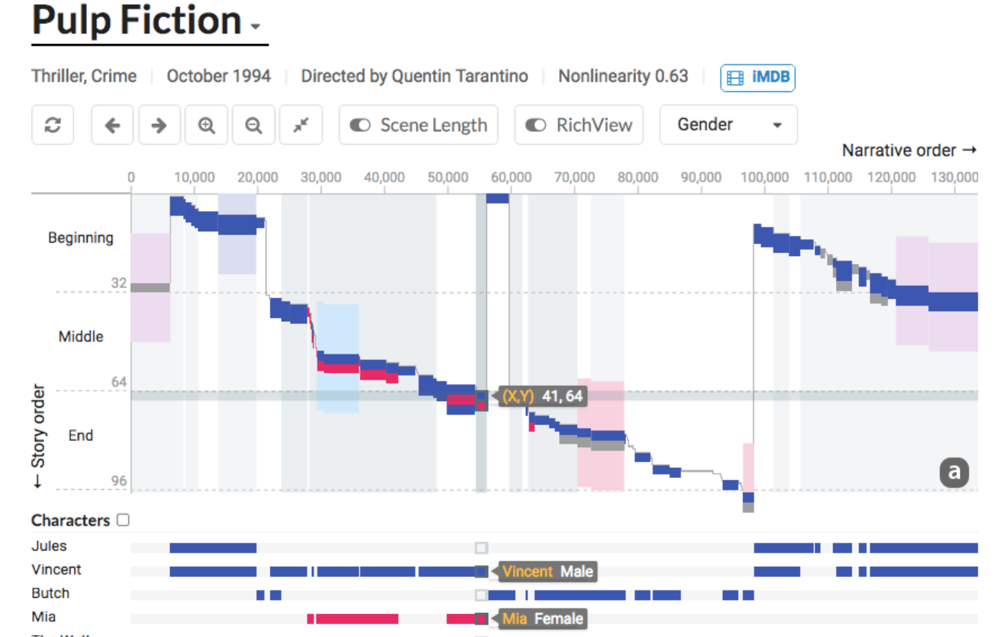{fig-alt="Story Curve for Pulp Fiction - from Kim et al (2018)" fig-align="center"}I used Python and [SpaCy](https://spacy.io/) together with [GLiNER](https://github.com/urchade/GLiNER) to extract characters, dates and places, and this mostly worked quite well. I then switched over to R for preprocessing and visualisation. I pulled down the Wikipedia character list to validate and match to the extracted ones (a good source of metadata). For the narrators, I used some formatting trickery, as they were in bold in the source text, but it needed a fair amount of manual fixing.My R code for the viz and initial results are below (click on a viz to zoom in). The locations are not quite right yet as I used some hacky approaches to extracting these. I'd like to turn these into interactives and include more of the character metadata and backstories in due course.*setup*```{r}#| label: Load Librariesoptions(tidyverse.quiet =TRUE)library(tidyverse)library(Polychrome)# prevent scientific notationoptions(scipen =999)# Set palettecolourCount =32# length(unique(timeline$id))newPalette =c("#000000", glasbey.colors(colourCount)[-1])names(newPalette ) <-NULL# Load Dataload(file ="timeline.RData")load(file ="narration.RData")```*story visualisation*```{r}#| label: Story Viz#| fig-height: 12#| fig-width: 18# Story Vizp1 <- timeline |>filter(label =="person") |>ggplot(aes(x = start + cum_position, y = year_corrected.x)) +geom_point(aes( colour = id, group = character),shape =15, size =2, position = ggstance::position_dodgev(height =1)) +geom_text(data = chaptersummaries, aes(x = cum_position + chlength/2, y =1999, label = chapter_corrected, ), check_overlap =TRUE, show.legend = F, size =6) +geom_text(data = chaptersummaries, aes(x = chlength/2+ cum_position, y = year_corrected, label = city),position =position_nudge(y =1),show.legend = F , check_overlap =TRUE, size =6) +geom_vline(data = chaptersummaries, aes(xintercept = chlength + cum_position), colour ="grey") +scale_color_manual(values = newPalette ) +scale_x_continuous(name ="position", limits =c(0, 300000)) +scale_y_reverse(name ="year", n.breaks =6) +theme_bw() +theme(legend.position ="none") +theme(plot.margin =margin(10, 10, 10, 90))```*character timeline*```{r}#| label: Character Viz# Character Vizp2 <- timeline |>filter(label =="person") |>group_by(id) |>#, chapter_correctedmutate(n =n()) |>mutate(first =min(start), last =max(end)) |>ggplot() +geom_segment(aes(x = start + cum_position, xend = end +400+ cum_position, y =reorder(character, n, decreasing = F) , yend = character, color = id), linewidth =5) +theme_bw() +geom_vline(data = chaptersummaries, aes(xintercept = chlength + cum_position), colour ="grey") +scale_color_manual(values = newPalette ) +scale_y_discrete(name ="Character") +scale_x_continuous(name ="Story Position", limits =c(0,300000)) +theme(legend.position ="none")```*narrators*```{r}#| label: Narrator Vizp3 <- narration |>ggplot() +geom_segment(aes(x = start + cum_position, xend =ifelse(is.na(endNarrate), end + cum_position, endNarrate + cum_position), y =reorder(character, desc(as.numeric(chapter))) , yend = character, color = id), linewidth =5) +theme_bw() +geom_vline(data = chaptersummaries, aes(xintercept = chlength + cum_position), colour ="grey") +#scale_color_manual(values = newPalette ) +scale_y_discrete(name ="Character") +scale_x_continuous(name ="Story Position", limits =c(0,300000)) +theme(legend.position ="none")``````{r}#| label: Lightboxed#| warning: false#| fig-cap: #| - Timeline, locations and characters#| - Character occurences#| - Narrators#| fig-height: 10#| fig-width: 18#| layout-nrow: 3#| lightbox: #| group: savage-chartsp1p2p3```


